SHOOTING METHOD

        Shooting method is one of the methods to solve the ordinary differential equation.

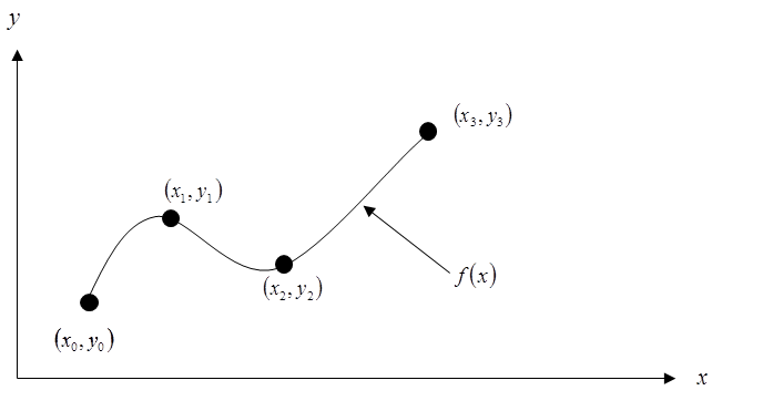
It is based on the boundary value problem where all the conditions are placed in the different points. We use trial approach and shoot one values and check for its solution in shooting method.

PROGRAM CODE

#include<iostream>

#include<cmath>

#include<cstdlib>

using namespace std;

float f1(float x,float y,float z){

    return(z);

}

float f2(float x,float y,float z){

    return(x+y);

}

float shoot(float x0,float y0,float z0,float xn,float h,int p){

    float x,y,z,k1,k2,k3,k4,l1,l2,l3,l4,k,l,x1,y1,z1;

    x=x0;

    y=y0;

    z=z0;

    do{

        k1=h*f1(x,y,z);

        l1=h*f2(x,y,z);

        k2=h*f1(x+h/2.0,y+k1/2.0,z+l1/2.0);

        l2=h*f2(x+h/2.0,y+k1/2.0,z+l1/2.0);

        k3=h*f1(x+h/2.0,y+k2/2.0,z+l2/2.0);

        l3=h*f2(x+h/2.0,y+k2/2.0,z+l2/2.0);

        k4=h*f1(x+h,y+k3,z+l3);

        l4=h*f2(x+h,y+k3,z+l3);

        l=1/6.0*(l1+2*l2+2*l3+l4);

        k=1/6.0*(k1+2*k2+2*k3+k4);

        y1=y+k;

        x1=x+h;

        z1=z+l;

        x=x1;

        y=y1;

        z=z1;

        if(p==1)

            cout<<endl<<x<<" "<<y;

    }while(x<xn);

    return(y);

}

int main(){

    float x0,y0,h,xn,yn,z0,m1,m2,m3,b,b1,b2,b3,e;

    int p=0;

    cout<<" Enter x, y, X, Y, h: "<<endl;

    cin>>x0>>y0>>xn>>yn>>h;

    cout<<" Enter trial M1 : ";

    cin>>m1;

    b=yn;

    z0=m1;

    b1=shoot(x0,y0,z0,xn,h,p=1);

    cout<<endl< " B1 = "<<b1<<endl;

    if(fabs(b1-b)<0.00005){

        cout<<"\n  The value of x and respective z are:\n";

        e=shoot(x0,y0,z0,xn,h,p=1);

        return(0);

    }else{

    cout<<" Enter trial M2 : ";

    cin>>m2;

    z0=m2;

    b2=shoot(x0,y0,z0,xn,h,p=1);

    cout<<endl< " B2 = "<<b2<<endl;

    }

    if(fabs(b2-b)<0.00005){

         cout<<"\n  The value of x and respective z are\n";

         e= shoot(x0,y0,z0,xn,h,p=1);

         return(0);

    }else{

    cout<<endl<<" M1 = <<m1<<" & M2 = "<<m2;

        m3=m2+(((m2-m1)*(b-b2))/(1.0*(b2-b1)));

        if(b1-b2==0)

        exit(0);

        cout<<"\nExact value of M = "<<m3;

        z0=m3;

        b3=shoot(x0,y0,z0,xn,h,p=0);

    }

    if(fabs(b3-b)<0.000005){

        cout<<"\nThere is solution :\n";

        e=shoot(x0,y0,z0,xn,h,p=1);

        exit(0);

    }

    do{

       m1=m2;

       m2=m3;

       b1=b2;

       b2=b3;

       m3=m2+(((m2-m1)*(b-b2))/(1.0*(b2-b1)));

       z0=m3;

       b3=shoot(x0,y0,z0,xn,h,p=0);

   }while(fabs(b3-b)<0.0005);

   z0=m3;

   e=shoot(x0,y0,z0,xn,h,p=1);

}

Note: This program is implemented in C++ using code blocks libraries.

LAGRANGIAN INTERPOLATION

           

            The lagrangian interpolation or lagrangian polynomials are perhaps the simplest way to exhibit the existence of a polynomial for interpolation with unequally spaced data. Data where the x-value is not equi-spaced often occurs as the result of experimental observation or when historical data are examined.

          The lagrangian polynomial equation is made up of  ‘n’ terms, each of which is a ‘n-1’ – ary degree where ‘n’ is the number of set of data. It, in fact passes through each point used in its construction.

SOURCE CODE

#include<iostream>

#include<cmath>

#include<iomanip>

using namespace std;

int main()

{

    double n,xx,mul;int i,j;

    int x[50],y[50];

    double sum=0;

    cout<<"input the value of n ";

    cin>>n;

    cout<<"enter the value of x and y:";

    for(i=0;i<n;i++)

    {

        cin>>x[i];

        cin>>y[i];

    }

cout<<"input point at which value is unknown:";

cin>>xx;

for(i=0;i<n;i++)

{

    mul=1;

    for(j=0;j<n;j++)

    {

        if(i!=j)

            mul=mul*(xx-x[i])/(x[i]-x[j]);

    }

sum=sum+mul*y[i];

}

cout<<"result="<<sum;

}

It can also be implemented as following:

#include<iostream>

using namespace std;

int main(){

    float *x, *y, result = 0, a;

    int size;

    cout<<"Enter the number of data : ";

    cin>>size;

    x = new float[size];

    y = new float[size];

    cout<<"Enter the data (x y):"<<endl;

    for (int i = 0; i < size; i++)

        cin>>x[i]>>y[i];

    cout<<"Enter the desired x : ";

    cin>>a;

    for (int i = 0; i < size; i++){

        float product = 1;

        for (int j = 0; j < size; j++){

            if(j != i)

                product *= ((a - x[j])/(x[i] - x[j]));

        }

        result += product*y[i];

    }

    cout<<"y("<<a<<") = "<<result<<endl;

    return 0;

}

RUNGE – KUTTA METHOD

            Runge – kutta(RK)  is also the one of the methods to solve the ordinary differential equation. This method does not require the calculation of higher order derivatives and gives greater efficiency. The RK formulae posses the advantages of requiring only the functional values at some selected points. These methods agree with Taylor’s series solution up to the h^r  term where ‘r’ differ from method to method and is called order of that methods. 

Source Code for RK Method

#include<iostream>

#include<cmath>

using namespace std;

float func(float x, float y){

    return -2*x-y;

}

int main(){

    float k[4]={0}, h=0.05, x=0.0, X=0.64, y=-1.0;  //f(0.6) = -0.846435

//    float k[4]={0}, h, x, y, X;

//    cout<<"Enter initial values of x (X0) and y (Y0) , final value of x (Xn) and the step value (h) :\n";

//    cin>>x>>y>>X>>h;

    do{

        y = y + (k[0]+2*k[1]+2*k[2]+k[3])/6;

        cout<<"f("<<x<<") =\t"<<y<<endl;

        k[0] = h*func(x,y);

        k[1] = h*func(x+h/2, y+k[0]/2);

        k[2] = h*func(x+h/2, y+k[1]/2);

        k[3] = h*func(x+h, y+k[2]);

        x = x + h;

    }while(x<=X);

    cout<<endl<<"f("<<X<<") = "<<y<<endl;

    return 0;

}

Source Code for RK-2 Method

#include<iostream>

using namespace std;

float func_f(float x,float y, float z)

{

    return z;

}

float func_g(float x,float y,float z)

{

    return -(x*z+y);

}

int main()

{

    float x=0.0, X=0.4, h=0.2, y=1, m[4], l[4], z=0.0;

    do

    {

        cout<<"("<<x<<", "<<y<<", "<<z<<")"<<endl;

        m[0]=func_f(x,y,z);

        l[0]=func_g(x,y,z);

        m[1]=func_f(x+h/2,y+(m[0]*h)/2,z+(l[0]*h)/2);

        l[1]=func_g(x+h/2,y+(m[0]*h)/2,z+(l[0]*h)/2);

        m[2]=func_f(x+h/2,y+(m[1]*h)/2,z+(l[1]*h)/2);

        l[2]=func_g(x+h/2,y+(m[1]*h)/2,z+(l[1]*h)/2);

        m[3]=func_f(x+h,y+(m[2]*h),z+(l[2]*h));

        l[3]=func_g(x+h,y+(m[2]*h)/2,z+(l[2]*h));

        y+=h*((m[0]+2*m[1]+2*m[2]+m[3])/6);

        z+=h*((l[0]+2*l[1]+2*l[2]+l[3])/6);

        x+=h;

    }while(x<=X);

    return 0;

}

Source Code for RK-4 Method

#include<iostream>

using namespace std;

float slope(float a,float b)

{

    return ((b-a)/(b+a));

}

int main()

{

    float x=0.0,x_n=1.0,h=0.2,y=1.0,k[4]={0.0};

    do

    {

        cout<<"("<<x<<","<<y<<")"<<endl;

        k[0]=h*slope(x,y);

        k[1]=h*slope(x+h/2,y+k[0]/2);

        k[2]=h*slope(x+h/2,y+k[1]/2);

        k[3]=h*slope(x+h/2,y+k[2]/2);

        y+=(k[0]+2*k[1]+2*k[2]+k[3])/6;

        x+=h;

    }while(x<=x_n);

    return 0;

}

EULER’S METHOD

        Euler’s method is one of the methods to solve the ordinary differential equation for first order equation.

The formula for Eulers method is given by:

          y_n+1=y_n+ h * f((x_n, y_n)

where,

          i= 1,2,3,4,……….

          h = step size

Source code for Euler’s method

#include<iostream>

#include<cmath>

using namespace std;

int main(){

    float x, X, y, n, h, m;

    cout<<"Enter initial value of x & y, final value of x and number of steps : "<<endl;

    cin>>x>>y>>X>>n;

    h = ( X - x ) / n;

    do{

        cout<<"f("<<x<<") = "<<y<<endl;

        m = ( y - x ) / ( y + x );

        y += m * h;

        x = x + h;

    }while(x<=X);

    return 0;

}

Source code for Modified Euler’s method

#include<iostream>

#include<cmath>

using namespace std;

int main(){

    float x, X, y, y1, Y, h, m, M;

    cout<<"Enter initial value of x & y, final value of x and stepping value :\n";

    cin>>x>>y>>X>>h;

    do{

        cout<<"f("<<x<<") = "<<y<<endl;

        M = ( y - x ) / ( y + x );  m = M;

        x = x + h;

        Y = y;

        do{

            y1 = y;

            y = Y + m * h;

            cout<<"f("<<x<<") = "<<y<<endl;

            m = ( y - x ) / ( y + x );

            m = ( M + m ) / 2;

        }while((abs(y1-y))>0.00004);

    }while(x<X);

    return 0;

}

LEAST SQUARE METHOD

Curve fitting is the process to fit a curve (or a function) to a given set of data. This method is useful to perform over inaccurate data. In this method, we fit a function to the experimental data that is unambiguous and that in some sense minimizes the deviations of the point from the function curve. The usual method for doing this is called the “least square method”. The deviations are determined by the distance between the points and the line of the function. How these distances are measured depends on whether there are experimental errors in both variables or in just one of them.

Source Code for least square method

         (for exponential equation)

// Example : a * e^b x

#include<iostream>

#include<cmath>

using namespace std;

int main()

{

 float *x, *y, sum_x=0, sum_y=0, sum_xy=0, sum_xx=0, del, del1, del2, a, b;

    int size;

  

 cout<<"Enter the size of data : ";

   cin>>size;

   x = new float[size];

   y = new float[size];

   

for (int i = 0; i < size; i++)

{

   

    cout<<"Enter the value of x and its respective y :";

 

      cin>>x[i]>>y[i];

     

  sum_x += x[i];

   

    sum_y += log(y[i]);

       sum_xx += x[i]*x[i];

 

      sum_xy += x[i]*log(y[i]);

   }

    del = pow(sum_x,2) - sum_xx*size;

   

del1 = sum_x*sum_y - sum_xy*size;

   

del2 = sum_x*sum_xy - sum_y*sum_xx;

  

 b = del1/del; a = exp(del2/del);

    cout<<"a = "<<a<<" and b = "<<b<<endl;

    return 0;

}

(for linear equation)

// Example : a * x + b

#include<iostream>

#include<cmath>

using namespace std;

int main(){

 float *x, *y, sum_x=0, sum_y=0, sum_xy=0, sum_xx=0, del, del1, del2, a, b;

    int size;

    cout<<"Enter the size of data : ";

    cin>>size;

    x = new float[size];

    y = new float[size];

    for (int i = 0; i < size; i++){

        cout<<"Enter the value of x and its respective y :";

        cin>>x[i]>>y[i];

        sum_x += x[i];

        sum_y += y[i];

        sum_xx += x[i]*x[i];

        sum_xy += x[i]*y[i];

    }

    del = pow(sum_x,2) - sum_xx*size;

    del1 = sum_x*sum_y - sum_xy*size;

    del2 = sum_x*sum_xy - sum_y*sum_xx;

    a = del1/del; b = del2/del;

    cout<<"a = "<<a<<" and b = "<<b<<endl;

    return 0;

}

Note: Above both programs are written in code blocks using C++ programming. 

POWER METHOD

Power method is used to find the dominant Eigen value and the corresponding Eigen vector. Eigen value problem generally arises in dynamics   programs and structural stability analysis. Power method is generally used to calculate these Eigen value and corresponding Eigen vector of the given matrix. This method can find only one Eigen value i.e. the greatest absolute value at a time.

          The utility of the power method is that it finds the Eigen-value of largest magnitude and its corresponding Eigen vector in a single and straight forward manner. It has the disadvantages that convergence is slow if there is a second Eigen value of nearly the same magnitude.

          The method works because e the Eigen vector is set of basis vectors. A set of basic vectors is said to be span the space, meaning the any x-component vector can be written as a unique linear combination of them.

Program code for Power method in C programming

(This program is written and compiled in TurboC++)

#include<stdio.h>

#include<math.h>

#define e 0.00001

int main()

{

    int n,i,j;

    float z[10],evaluemax,eigenvector[20][20],eigenvalue=0,sum,y[10], a[20][20],x[10],error;

    printf("Enter number  of equations");

    scanf("%d",&n);

    printf("Enter augumented matrix");

    for(i=1;i<=n;i++)

    {

        for(j=1;j<=n+1;j++)

        {

            printf("a[%d][%d]=",i,j);

            scanf("%d",&a[i][j]);

        }

    }

    printf("Enter initial guess for eigen vector");

    {

        for(i=1;i<=n;i++)

        {

            for(j=1;j<=1;j++)

            {

                scanf("%d",&eigenvector[i][j]);

            }

        }

    }

    do

    {

    for(i=1;i<n;i++)

    {

        x[i]=a[i][n+1]/a[i][i];

    }

    do

    {

    for(i=1;i<=n;i++)

    {

        sum=0;

        for(j=1;j<=1;j++)

        {

            if(i!=j)

                sum=sum+a[i][j]*x[j];

        }

        z[i]=sum;

    }

    }

    evaluemax=fabs(z[i]);

    for(i=1;i<=n;i++)

    {

        if(evaluemax<z[i])

            evaluemax=z[i];

    }

    while(error>e);

     error=fabs(eigenvalue-evaluemax);

     eigenvalue=evaluemax;

     printf("Eigen value and eigen vector %d", x[i]);

    }

Program code for Power method in C++ programming

(This program is written and compiled in code blocks)

#include<iostream>

#include<cmath>

using namespace std;

float findMax(float *arr, int size){

    float max = fabs(arr[0]);

    for (int i = 1; i < size; i++){

        if ( max < fabs(arr[i]))

            max = fabs(arr[i]);

    }

    return max;

}

int main(){

    float mat[30][30], vect[30], lem, z[30], sum, check;

    int size;

    cout<<"Enter the size of matrix (<30):";

    cin>>size;

    cout<<"Enter the matrix :"<<endl;

    for (int i = 0; i < size; i++){

        for (int j = 0; j < size; j++)

            cin>>mat[i][j];

    }

    cout<<"Enter the vector :"<<endl;

    for (int i = 0; i < size; i++)

        cin>>vect[i];

    do{

        for (int i = 0; i < size; i++){

            sum = 0;

            for (int j = 0; j < size; j++){

                sum += mat[i][j]*vect[j];

            }

            z[i] = sum;

        }

        lem = findMax(z, size);

        for (int i = 0; i < size; i++)

            z[i] /= lem;

        float diff[30];

        for (int i = 0; i < size; i++)

            diff[i] = vect[i]-z[i];

        check = findMax(diff, size);

        for (int i = 0; i < size; i++)

            vect[i] = z[i];

   }while(check > 0.1);

    cout<<"The required value is : "<<lem<<endl;

    return 0;

}